The code to run these plots reside in the visualization repository
Spatial IM plots
1. Generate summary csv and meta info file using https://github.com/ucgmsim/IM_calculation/blob/master/calculate_ims.py. For further info please refer to IM Calculation Refactor
2. Identify a station.ll file or a rrup.csv file that contains station and coordinates information
3. Generate .xyz files using https://github.com/ucgmsim/visualization/blob/im_plot/im_plotting/im_plot.py with the following input: (1) summary csv in step 1; (2) station file in step 2.
4. Generate IM plots pngs using https://github.com/ucgmsim/visualization/blob/im_plot/gmt/plot_stations.py
Note: Step 3 is based on the assumptions that (1) summary csv and meta info files are in the same dir; (2) summary csv and meta info files have the same prefix
usage: im_plot.py [-h] [-o OUTPUT_PATH] [-c COMPONENT]
                  csv_filepath rrup_or_station_filepath
positional arguments:
  csv_filepath          path to input csv file
  rrup_or_station_filepath
                        path to inpurt rrup_csv/station_ll file path
optional arguments:
  -h, --help            show this help message and exit
  -o OUTPUT_PATH, --output_path OUTPUT_PATH
                        path to store output xyz files
  -c COMPONENT, --component COMPONENT
                        which component of the intensity measure. Available
                        compoents are ['geom', '090', '000', 'ver']. Default
                        is 'geom'
Example:
To generate .xyz
python im_plot.py ~/kelly_sim_ims/kelly_sim_ims.csv /home/nesi00213/dev/impp_datasets/Darfield/sample_nz_grid.ll -o ~/xyz_test
To plot pngs
python plot_stations.py ~/xyz_test/nonuniform_im_plot_map_kelly_sim_ims.xyz --out_dir ~/xyz_test --model_params /home/nesi00213/VelocityModel/v1.64_FVM/model_params_nz01-h0.100
--srf /home/nesi00213/RunFolder/Cybershake/v18p6/verification/Kelly/Kelly_HYP03-29_S1264.srf
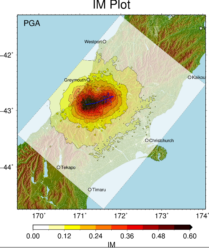
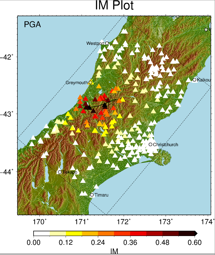
Sample nonuniform plot Sample uniform plot
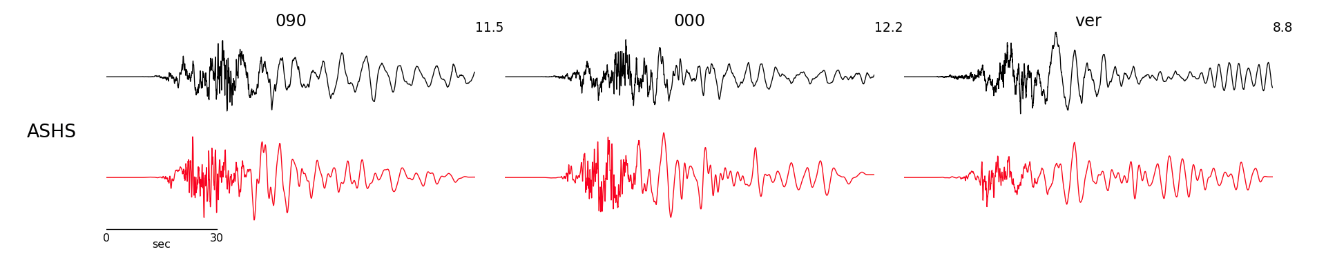
Waveform Time Series
 usage: waveforms_sim_obs.py [-h] [--sim-prefix SIM_PREFIX]
                            [--obs-prefix OBS_PREFIX] [-v] [-n NPROC]
                            sim obs out
positional arguments:
  sim                   path to binary file or text dir for simulated
                        seismograms
  obs                   path to text dir for observed seismograms
  out                   output folder to place plots
optional arguments:
  -h, --help            show this help message and exit
  --sim-prefix SIM_PREFIX
                        sim text files are named <prefix>station.comp
  --obs-prefix OBS_PREFIX
                        obs text files are named <prefix>station.comp
  -v                    verbose messages
  -n NPROC, --nproc NPROC
                        number of processes to use
IM vs Rupture Distance
usage: im_rrup.py [-h] [--out-dir OUT_DIR] [--run-name RUN_NAME] [--im IM]
                  [--comp COMP]
                  rrup
positional arguments:
  rrup                 path to RRUP file
optional arguments:
  -h, --help           show this help message and exit
  --out-dir OUT_DIR    output folder to place plot
  --run-name RUN_NAME  run_name - should automate?
  --im IM              path to IM file, repeat as necessary
  --comp COMP          component
pSA station
usage: psa_sim_obs.py [-h] [-s SIM] [-o OBS] [-d OUT_DIR]
 [--run-name RUN_NAME] [--comp COMP]
optional arguments:
 -h, --help show this help message and exit
 -s SIM, --sim SIM path to SIMULATED IM file
 -o OBS, --obs OBS path to OBSERVED IM file
 -d OUT_DIR, --out-dir OUT_DIR
 output folder to place plots
 --run-name RUN_NAME run_name - should automate?
 --comp COMP component