This page has descriptions of the file formats that we use in various places.
| Table of Contents |
|---|
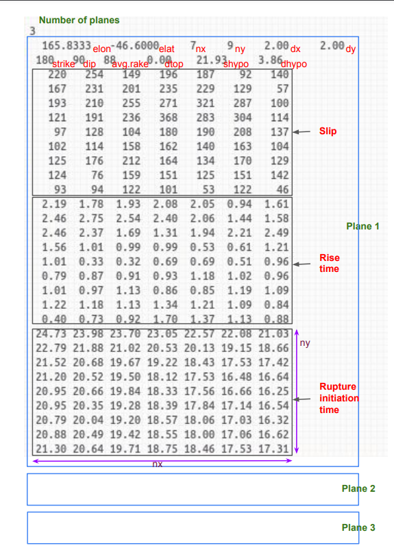
SRF Format
- https://strike.scec.org/scecpedia/Standard_Rupture_Format
- SRF-Description-Graves_2.0.pdf
- SRF File Format Version 1 (output of genslip): srf_description_version_1.pdf
- Details on Source Modelling : Source Modelling for GMSim
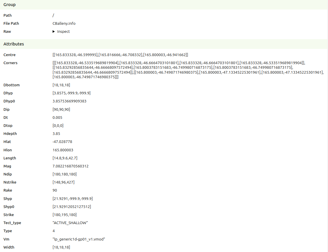
SRF info format
The .info files that accompany .srf files are in HDF5 format
Example (CBalleny.info)
Stoch format
LF/HF/BB binary format
These files store timeseries data. All formats follow a style derived from the LF seis format produced by EMOD3D:
...
| LF | HF | BB |
|---|---|---|
i4 number of stations TOTAL 4 BYTES | i4 number of stations
i4 number of ray methods
i4 first ray method used TOTAL 288 BYTES | i4 number of stations TOTAL 788 BYTES |
START OFFSET 4 BYTES i4 index of station in input file TOTAL 48 BYTES * NUM_STATIONS | START OFFSET 512 BYTES f4 longitude of station (degrees) TOTAL 24 BYTES * NUM_STATIONS | START OFFSET 1280 BYTES f4 longitude of station (degrees) TOTAL 44 BYETS * NUM_STATIONS |
START OFFSET 0 FROM ABOVE f4 velocity (cm/s) timeseries in array dimensions: TOTAL 4 BYTES * PRODUCT_OF_DIMENTIONS | START OFFSET 0 FROM ABOVE f4 acceleration (cm/s^2) timeseries in array dimensions: TOTAL 4 BYTES * PRODUCT_OF_DIMENTIONS | START OFFSET 0 FROM ABOVE f4 acceleration (g) timeseries in array dimensions: TOTAL 4 BYTES * PRODUCT_OF_DIMENTIONS |
XYTS.e3d binary format
This file is produced by EMOD3D and contains a timeseries of ground motions on the XY plane. Unlike the LF seis files, this contains data at all grid points and may have a decimated resolution specified when running EMOD3D through the e3d.par file with the parameters dxts and dyts.
Numbers are 4 bytes in length and may be little or big endian. You can see or use the existing interfaces that also take care of endianness at github:ucgmsim/qcore/qcore/xyts.py::XYTSFile.
File size can be derived knowing the format and the shape of time-series (all necessary values are at the beginning of the file).
...
- simulation metadata
- INTEGERS
- number of first x gridpoint
- number of first y gridpoint
- number of first z gridpoint
- number of first timestep
- number of x gridpoints
- number of y gridpoints
- number of z gridpoins (always 1 by definition of X-Y file)
- number of timesteps
- FLOATS
- x spacing between given gridpoints (km)
- y spacing between given gridpoints (km)
- original (pre-decimated) grid spacing between gridpoints used in simulation (km)
- timestep in timeseries (s)
- model rotation of gridpoints (degrees)
- model centre latitude (degrees)
- model centre longitude (degrees)
- x spacing between given gridpoints (km)
- INTEGERS
- timeseries
- float array of velocities in the dimentions of timesteps, components (x, y, z), y grid positions, x grid positions.
Intensity Measure calculation
The IM calculation code will produce a number of text files (decided as of 25/05/2018). We will summarize them in the following.
Intensity measure files
There are two types of IM files: per station and aggregate. The per station one has the following format:
...
| Code Block |
|---|
station, component, IM_1, IM_2, ...., IM_N |
Empirical IMs
As above the empirical intensity measures have a similar format:
...
Notes: 1) the component for empirical IMs is always 'geom' 2) only total sigma is saved to the csv file
Rrup file
The file format for this is:
...
Note: we don't have rx calculations yet, so we may dump an invalid value just to conform with the format.
Metadata file
So far the requirements indicate that we need:
| Code Block |
|---|
identifier, rupture, type, date, version |
GSF File
The GSF file is used to define the geometry of a source in a source modelling problem. It is the first step in the SRF generation process after a realisation is read.
A GSF file contains three sections in order:
- Errata/Header section,
- Declaration of the number of points (N),
- The geometry description: N lines representing each point in the geometry.
There are utilities to read GSF files in the gsf module within qcore.
Example File
Below is a discretisation of the Acton fault. You can visualise this gsf file use the gsf_plot script in the visualisation repo under the sources folder.
| View file | ||||
|---|---|---|---|---|
|
Errata/Header
The header consists of a number of commented lines, each beginning with # . Here is an example:
| Code Block |
|---|
# nstk= 179 ndip= 215
# flen=    17.0720 fwid=   21.2853
# LON LAT DEP(km) SUB_DX SUB_DY LOC_STK LOC_DIP LOC_RAKE SLIP(cm) INIT_TIME SEG_NO |
This is the typical output of fault_seg2gsf . The first line has the number of points in the strike and dip directions, respectively. Then the length and width of the fault, and the last line is a description of each column in the points section.
The header is skipped by programs parsing GSF files and may contain any number of lines. The Python GSF generator, for example, only prints out the column description.
| Code Block |
|---|
# LON LAT DEP(km) SUB_DX SUB_DY LOC_STK LOC_DIP LOC_RAKE SLIP(cm) INIT_TIME SEG_NO |
Declaration of the Number of Points
Immediately following the header, there is one line containing the number of points in the GSF geometry definition.
Geometry Description
The geometry description has N lines, where N is the number of points declared in the previous section. Each line has 11 space separated values representing one point in the geometry.
| Column | Description |
|---|---|
| LON | The longitude of the point. |
| LAT | The latitude of the point. |
| DEP | The depth of the point (in kilometres, with 10 meaning 10km below ground level). |
| SUB_DX | The subdivision length in the strike direction. |
| SUB_DY | The subdivision length in the dip direction. |
| LOC_STK | The fault plane strike. |
| LOC_DIP | The fault plane dip. |
| LOC_RAKE | The fault plane rake. |
| SLIP | The total slip at this point (cm), usually -1. |
| INIT_TIME | The initial rupture time of this point, usually -1. |
| SEG_NO | The number corresponding to the segment this point belongs to.: |
Here an example of a line from the Acton fault GSF file.
168.36970 -45.45649 6.04586e-01 9.58498e-02 9.94142e-02 196.0 60.0 110.0 -1.00 -1.00 0
Point Order
The order of the points is important! The points must be in order of first strike and then dip. That is to say, first every point on all planes at depth = 0 should be written, then depth = 1, depth = 2, and so on and the order of the points at a fixed depth = i is in order of strike. Refer to the diagram below.
