Processing observed data for 4 recorded events

TO DO: To have a proper low frequency data required for solving tomography problem, we need to list the specific stations recording the event from a general station list of the Canterbury region; re-sample the recorded seismogram to expected sampling rate; shift the recorded data based on the given time shift; and filter the data to the frequency band interested.

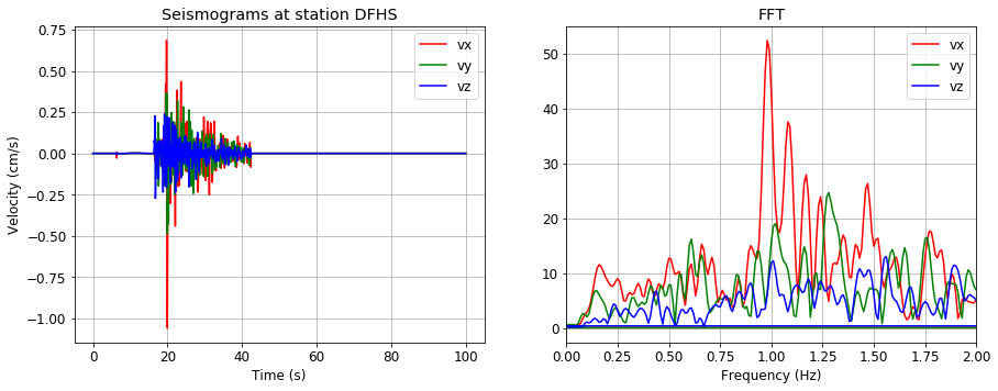
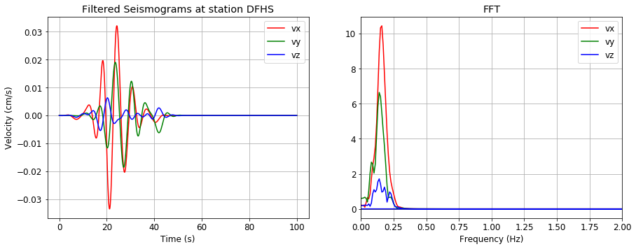
Example of recorded data before and after applying filter from 0-0.2Hz for event 3550173m4pt7 at station DFHS

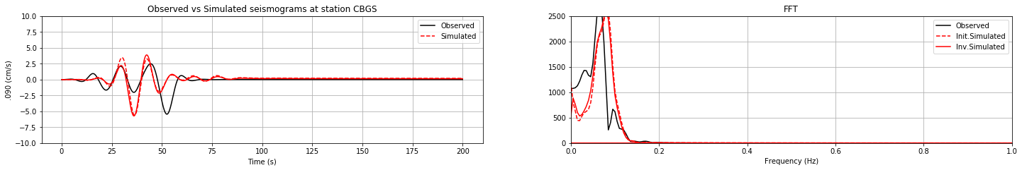
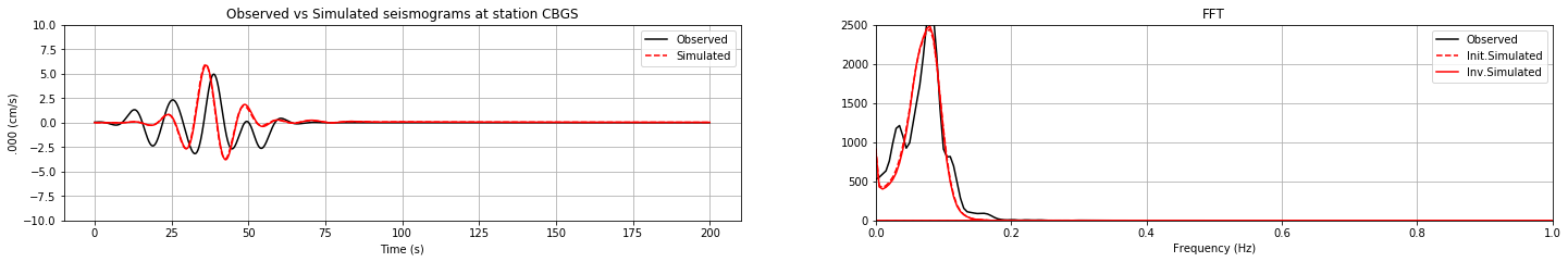
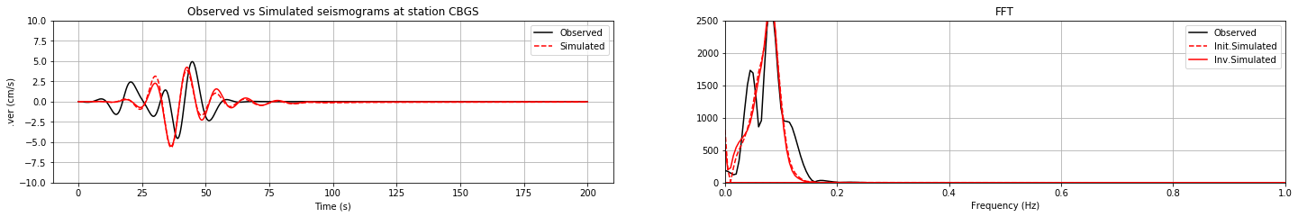
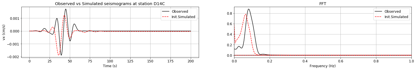
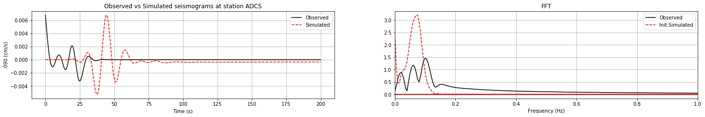
Comparison between the observed seismogram and seismogram simulated using emod3d with srf source for a homogeneous model; both are filtered from 0-0.1Hz

Quantify waveform similarity between synthetic and observed seismograms for 78 stations according to event 3550173m4pt7 using normalized correlation coefficient (NCC) defined as

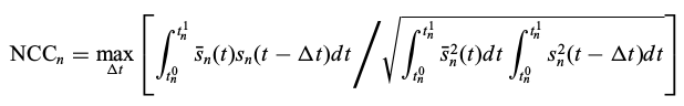
Here, the synthetic seismograms are generated using srf source for a homogeneous model of Vs=3.0km/s, Vp=6.0 km/s

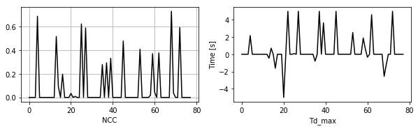
Example of removing low-quality observed seismograms with NCC<0.2

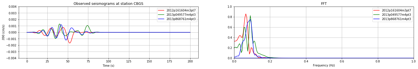
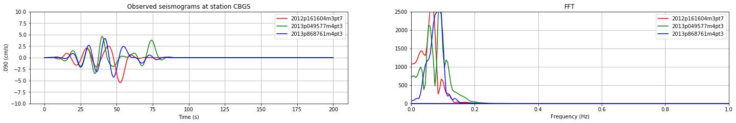
Normalize the observed seismogram (filtered from 0-0.1 Hz) at a station for 3 different events:

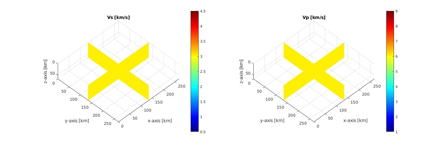
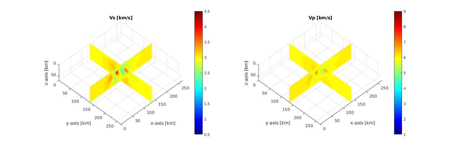
First inversion of the Canterbury velocity  model using gsdf broad band selection of the adjoint source for 4 frequencies [0.025 0.05 0.075 0.1] Hz and observed seismograms from 4 earthquake events: 2012p161604m3pt7, 2013p049577m4pt3, 2013p868761m4pt3, 3550173m4pt7

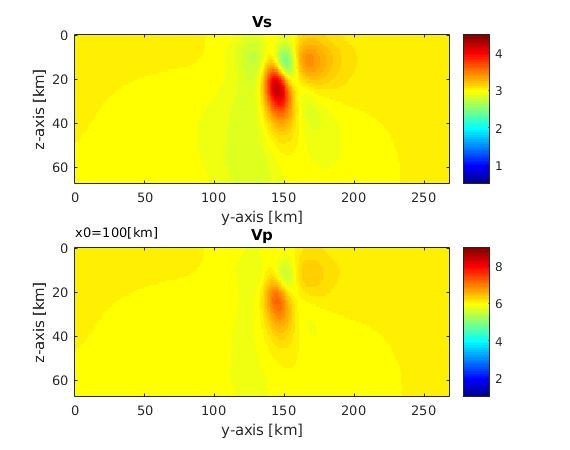
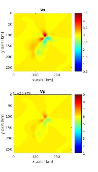
Cross-sections of the inverted model

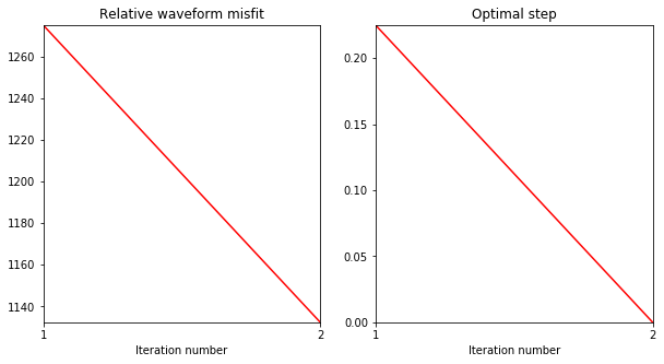
Misfit function and step length:

Waveform comparison between observed and simulated seismograms after one iteration for event 2012p161604m3pt7